Top Solutions for Kaggle Quantitative Competitions¶

1 Introduction¶

Recently, quantitative competitions have emerged one after another on Kaggle.
There is Jane Street's competition predicting trades and maximizing profits, the Optiver competition predicting realized volatility just ended. There are also ongoing competitions, such as G-Research's competition for forecasting cryptocurrency returns and Jiu-Kun's competition for predicting returns by domestic quantitative private equity firms.
Maybe these institutions have really gained many insights from Kaggle and earned a lot of money, which makes them so enthusiastic about holding such competitions.
Unlike previous interpretations of solutions released during the competition:

• Want to Experience Quantitative Trading
• Copying Homework

This article will interpret the final top solutions for the Jane Street Market Prediction and Optiver Realized Volatility Prediction competitions.

2 Competition Overview¶

Let's briefly review the two competitions:

• Jane Street requires us to provide trading signals to maximize profits.
• Optiver requires us to predict the volatility of high-frequency financial data (stocks).

During the Private Leaderboard phase of both competitions, actual financial data is regularly used to update the rankings of the solutions. Although financial markets are difficult to predict, miraculously, high-scoring teams can keep themselves at the top of the leaderboard, making people have to agree on the effectiveness of their solutions. Let's take a look at their winning solutions together.

3 Solution Interpretation¶

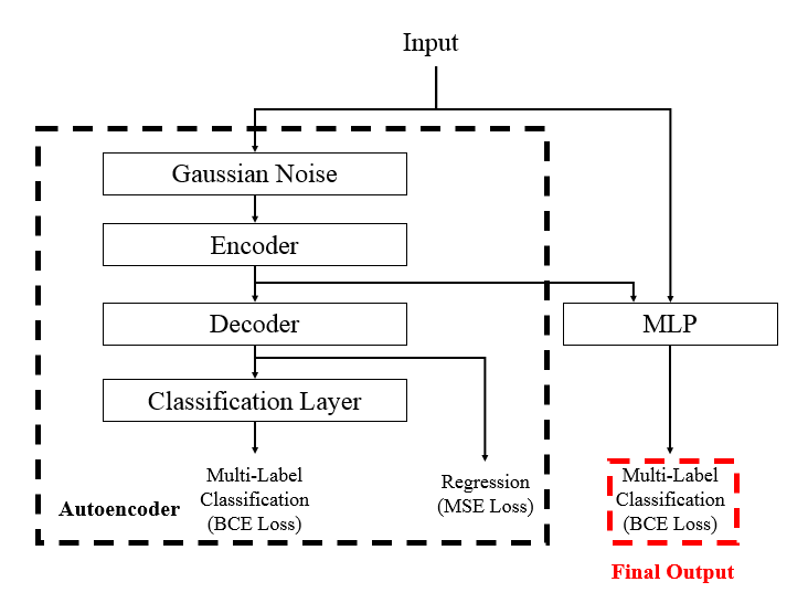
3.1 Jane Street Top 1 solution from Cats Trading...¶

The winning solution used an XGBoost model and a neural network (Supervised Autoencoder with MLP) model with an autoencoder, of which the latter single model can also maintain first place. The model structure is shown below:

def create_ae_mlp(num_columns, num_labels, hidden_units, dropout_rates, ls = 1e-2, lr = 1e-3):

    inp = tf.keras.layers.Input(shape = (num_columns, ))
    x0 = tf.keras.layers.BatchNormalization()(inp)

    encoder = tf.keras.layers.GaussianNoise(dropout_rates[0])(x0)
    encoder = tf.keras.layers.Dense(hidden_units[0])(encoder)
    encoder = tf.keras.layers.BatchNormalization()(encoder)
    encoder = tf.keras.layers.Activation('swish')(encoder)

    decoder = tf.keras.layers.Dropout(dropout_rates[1])(encoder)
    decoder = tf.keras.layers.Dense(num_columns, name = 'decoder')(decoder)

    x_ae = tf.keras.layers.Dense(hidden_units[1])(decoder)
    x_ae = tf.keras.layers.BatchNormalization()(x_ae)
    x_ae = tf.keras.layers.Activation('swish')(x_ae)
    x_ae = tf.keras.layers.Dropout(dropout_rates[2])(x_ae)

    out_ae = tf.keras.layers.Dense(num_labels, activation = 'sigmoid', name = 'ae_action')(x_ae)

    x = tf.keras.layers.Concatenate()([x0, encoder])
    x = tf.keras.layers.BatchNormalization()(x)
    x = tf.keras.layers.Dropout(dropout_rates[3])(x)

    for i in range(2, len(hidden_units)):
        x = tf.keras.layers.Dense(hidden_units[i])(x)
        x = tf.keras.layers.BatchNormalization()(x)
        x = tf.keras.layers.Activation('swish')(x)
        x = tf.keras.layers.Dropout(dropout_rates[i + 2])(x)

    out = tf.keras.layers.Dense(num_labels, activation = 'sigmoid', name = 'action')(x)

    model = tf.keras.models.Model(inputs = inp, outputs = [decoder, out_ae, out])
    model.compile(optimizer = tf.keras.optimizers.Adam(learning_rate = lr),
                  loss = {'decoder': tf.keras.losses.MeanSquaredError(),
                          'ae_action': tf.keras.losses.BinaryCrossentropy(label_smoothing = ls),
                          'action': tf.keras.losses.BinaryCrossentropy(label_smoothing = ls),
                         },
                  metrics = {'decoder': tf.keras.metrics.MeanAbsoluteError(name = 'MAE'),
                             'ae_action': tf.keras.metrics.AUC(name = 'AUC'),
                             'action': tf.keras.metrics.AUC(name = 'AUC'),
                            },
                 )

    return model

It can be seen that the final loss is the MSE loss of the decoder plus the BCE loss of the autoencoder (whether to trade) plus the BCE loss of the spliced network after the original input and the encoder spliced. Although there were open-source solutions using autoencoders during the competition, Cats Trading... optimized the autoencoder part and the spliced network at the same time, thereby avoiding leakage caused by training the autoencoder first and then using CV(cross-validation).

3.2 Optiver Top 1 solution from nyanp¶

As mentioned in previous articles, the data provided by the competition mainly includes two categories of trading-related data (prices,

Comments