Analysis of Variance (ANOVA)¶

1 Introduction¶

Last time, I talked about choosing the minimum sample size which focuses more on testing the mean and ratio of single or two samples. For the mean test of multiple samples, we can use ANOVA (Analysis of Variance) to analyze it separately.

Before we start, let's consider a question: since we already have the universal and useful AB test, why do we still need ANOVA? The answer is simple. In a production environment, the dependent variables we are interested in are usually influenced by many factors. For example, the effectiveness of a new drug is influenced by conditions such as indications, dosage, route and method of administration, and daily frequency of administration. Similarly, the sales of a product are influenced by factors such as advertising, product price, seasonal changes, etc. In addition, each influencing factor may have multiple observation levels. For example, the UI design of a webpage may have multiple versions, labeled as ABCDEFG (after all, black does not necessarily mean the same black). When the boss asks you whether these factors have an impact on the dependent variable and whether there are significant differences in the observation values of each level of the factor, relying solely on the two levels of the single factor AB test will be insufficient. Unless we combine every possible combination and test all of them, however, multiple tests will increase the probability of making Type I errors and it is impossible to consider all samples simultaneously. This is where ANOVA comes in to save the day.

2 Principle Introduction¶

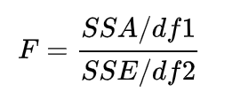
In the case of a single factor, ANOVA is actually used to compare whether the means of multiple sample sets are the same/whether multiple sample sets have the same distribution. So why call it "Analysis of Variance"? Simply put, it comes from the decomposition of errors. We use the sum of squares of deviations of samples to measure the total error of the population, where the total error SST (Sum of Square for Total) = random error in the group SSE (Sum of Square for Error) + error between the groups SSA (Sum of Square for factor A). The statistical quantities are shown below. SSE divided by its degrees of freedom is equivalent to the variance of each group, and SSA divided by its degrees of freedom is equivalent to the variance of each group relative to the total population. When the sample follows a normal distribution, the sum of squares of deviations follows a chi-square distribution, so this statistical quantity is equivalent to the ratio of two chi-square distributions, which is a distribution of F. When the F-statistic is larger, it indicates that the denominator is small, the within-group variance is small, and they are tightly concentrated; the numerator is large, the between-group variance is large, the groups are far apart, and it tends to reject the null hypothesis of the equal means/distributions of multiple samples.

ANOVA has many variations and can be divided into one-way ANOVA and multi-factor ANOVA according to the number of factors. When related to experimental design DOE (Design of Experiment), there are many forms like completely random design, randomized block design, Latin square design, orthogonal design, etc. But great wisdom is simple, and different paths lead to the same destination. As long as you master the basic logic of ANOVA, you can easily handle all kinds of variations. Here we mainly classify according to the number of factors. Sure! Here’s your translation with the same markdown format preserved:

2.1 One-Way Analysis of Variance (One Way ANOVA)¶

One-way ANOVA focuses on a single influencing factor, which may have multiple levels. For example, the impact of three UI design versions (A, B, C) on traffic mentioned earlier — here, UI design is the factor, and the three versions A, B, C are the three levels of this factor. The specific testing process is as follows:

• Establish null and alternative hypotheses: Typically, the null hypothesis assumes that the means of all groups are equal, and the alternative hypothesis assumes that at least one mean is different.
• Calculate the F-statistic: Compute group means, overall mean, the sums of squares of errors, and degrees of freedom to obtain the F-statistic.
• Draw the conclusion: Compare the F-statistic with the critical value from the F-distribution table. If the F-statistic is greater than the critical value, the null hypothesis can be rejected, indicating that there is a difference among the group means. Alternatively, you can calculate the p-value and compare it with a pre-set significance level α. If the p-value is less than α, the null hypothesis is rejected.
• Post-hoc analysis: This is a pairwise comparison analysis. After rejecting the null hypothesis in the previous step, it indicates that at least one group mean is different. Tukey's test or Bonferroni test can be used for pairwise comparisons to identify which groups have significant differences.

Example: Simulating data since no real experimental data is available.

import numpy as np
# Simulate a one-factor three-level dataset: control group and two experimental groups
# The mean of treat1 is very close to the control group, while treat2 differs significantly
df = {'control': list(np.random.normal(10, 5, 100)),
      'treat1': list(np.random.normal(11, 5, 100)),
      'treat2': list(np.random.normal(20, 5, 100))}

import pandas as pd
# Convert to DataFrame
df = pd.DataFrame(df)
df.head()

# Reshape the dataset for ANOVA
df_melt = df.melt()
df_melt.head()
df_melt.columns = ['Treat', 'Value']
df_melt.head()

# Visualize with boxplot
import seaborn as sns
sns.boxplot(x='Treat', y='Value', data=df_melt)

from statsmodels.formula.api import ols
from statsmodels.stats.anova import anova_lm
# One-way ANOVA example. For multi-factor, use Value~C(factor1)+C(factor2)...
# If there is interaction between factors, add interaction terms like C(factor1):C(factor2)
model = ols('Value~C(Treat)', data=df_melt).fit()
anova_table = anova_lm(model, typ=2)
print(anova_table)

# Equal sample sizes, so Tukey's test can be used for pairwise comparisons
from statsmodels.stats.multicomp import MultiComparison
mc = MultiComparison(df_melt['Value'], df_melt['Treat'])
tukey_result = mc.tukeyhsd(alpha=0.5)
print(tukey_result)

The simulation results show that the p-value for this factor tends towards 0, and the F-statistic is large, allowing us to significantly reject the null hypothesis. The post-hoc pairwise comparison shows no significant difference between the control group and treat1, but treat2 differs significantly from both other groups.

2.2 Multi-Factor Analysis of Variance (MANOVA)¶

MANOVA examines two or more influencing factors. For instance, product sales may be influenced by both price and advertising. Price and advertising are two factors, each with multiple levels. We want to determine whether these factors significantly affect product sales.

import numpy as np
# Simulate a two-factor dataset: one factor has 3 levels, the other has 5 levels
data = np.array([
    [276, 352, 178, 295, 273],
    [114, 176, 102, 155, 128],
    [364, 547, 288, 392, 378]
])
df = pd.DataFrame(data)
# Set factor names
df.index = pd.Index(['A1', 'A2', 'A3'], name='ad')
df.columns = pd.Index(['B1', 'B2', 'B3', 'B4', 'B5'], name='price')
print(df)

# Reshape the dataset for ANOVA
df1 = df.stack().reset_index().rename(columns={0: 'value'})
print(df1)

from statsmodels.formula.api import ols
from statsmodels.stats.anova import anova_lm
# Two-way ANOVA
# If there is interaction between factors, add interaction terms like C(factor1):C(factor2)
model = ols('value~C(ad) + C(price)', df1).fit()
anova_table = anova_lm(model)
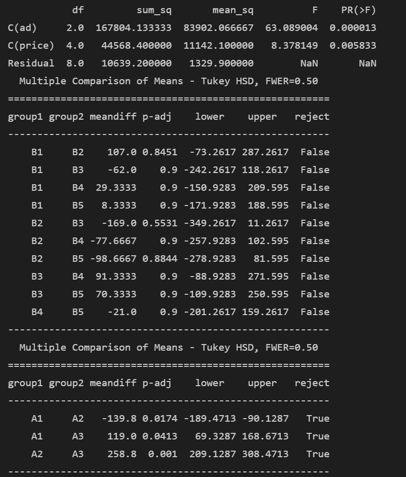
print(anova_table)

# Equal sample sizes, so Tukey's test can be used for pairwise comparisons
from statsmodels.stats.multicomp import MultiComparison
mc = MultiComparison(df1['value'], df1['price'])
tukey_result = mc.tukeyhsd(alpha=0.5)
print(tukey_result)

mc2 = MultiComparison(df1['value'], df1['ad'])
tukey_result2 = mc2.tukeyhsd(alpha=0.5)
print(tukey_result2)

The simulation results show that both the price and advertising factors have small p-values and large F-statistics, allowing us to significantly reject the null hypothesis, indicating both factors have a significant impact on product sales. The post-hoc pairwise comparison shows no significant difference among prices, but significant differences among advertisements.

2.3 Conditions for Use¶

The conditions for applying ANOVA are: - Homogeneity of variances: Use Bartlett's test to check for variance homogeneity. If homogeneity cannot be rejected, proceed with ANOVA. If heterogeneity is found, you can adjust using methods like Welch's correction before performing ANOVA. - Observations are independently and identically distributed (i.i.d). - Observations follow a normal distribution: If not, non-parametric tests can be used.

3 Summary¶

For ANOVA, as long as you clearly define the research subject and experimental design, the following steps will proceed smoothly. The core is to use the F-test to compare inter-group variance and intra-group variance. Have you got it?

Comments